1. Introduction
In quantum information, a lot of information is included in the phase of the quantum state. The quantum Fourier transform algorithm introduced in quantum fourier transform can be used to generalize and construct the quantum phase estimation algorithm. The quantum phase estimation algorithm (or quantum eigenvalue estimation algorithm) can estimate the eigenvalue of an eigenstate corresponding to a unitary operator up to certain precision. Specifically $U$ is a unitary transformation in the Hilbert space of $n$ qubits. The operator $U$ corresponds to an eigenstate $|\psi\rangle$ with eigenvalue $e^{2 \pi i \varphi}$, i.e.
\begin{equation}
U|\psi\rangle=e^{2 \pi i \varphi}|\psi\rangle\label{327}
\end{equation}
where the value of $0\leq \varphi < 1$ is unknown. The quantum phase estimation algorithm is to give a finite accurate estimate for $\varphi$ by performing a series of controlled gates such as controlled $U$, controlled $U^{2^1}$, controlled $U^{2^2}$, and so on. That is, the estimate for $\varphi$ is accurate to $L$ bits.
2. Overview (in math) For the quantum phase estimation algorithm the quantum register consists of two parts, the first part of the register consists of $L$ qubits whose initial state is $|0\rangle$ and these $L$ qubits are responsible for estimating the phase. The exact amount of $L$ depends on the precision of the desired phase estimation and the desired success rate of the phase estimation process. The second part of the register is used to input the eigenstate $|\psi\rangle$ of the phase being estimated. The dimension of the second part of the register should be equal to the dimension of the eigenstate $|\psi\rangle$.
The first stage quantum circuit of the quantum phase estimation algorithm is shown in Figure 1.
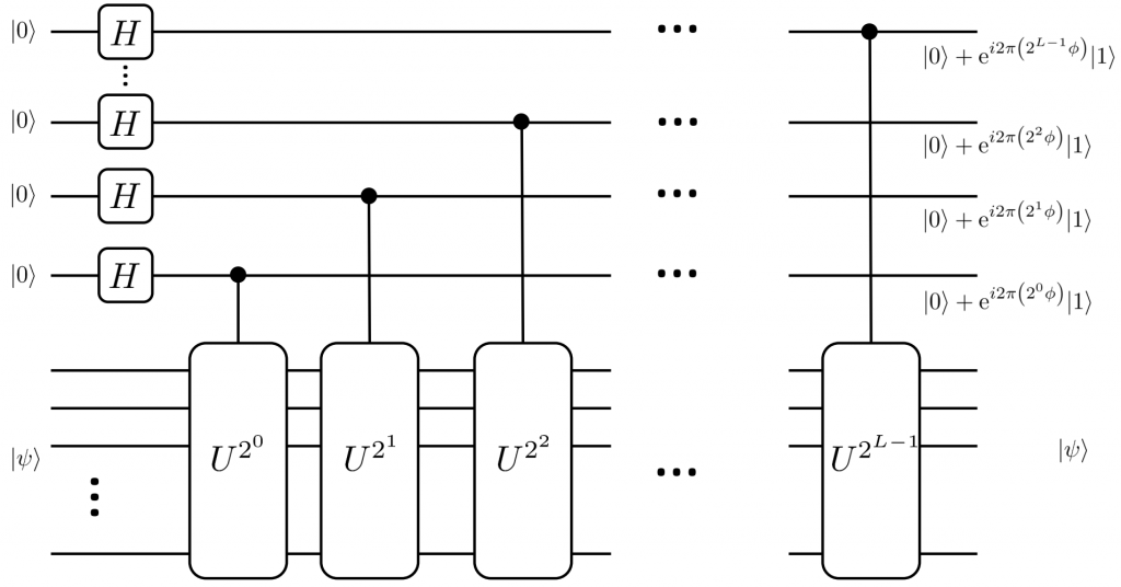
Figure 1: Quantum circuit of phase estimation algorithm subroutin I
First the initial state $|0\rangle^{\otimes L}|\psi\rangle$ is prepared. Afterwards perform $L$-qubit Hadamard gate $H^{\otimes L}$ for the first quantum memory $L$-qubit:
\begin{equation}
\frac{1}{2^{L/2}}\left(|0\rangle+|1\rangle\right)^{\otimes L}|\psi\rangle
\end{equation}
$U|\psi\rangle=e^{2 \pi i \varphi}|\psi\rangle$ in the quantum circuit, thus
\begin{equation}
U^{2^{j}}|\psi\rangle=U^{2^{j}-1}U|\psi\rangle=U^{2^{j}-1}e^{2 \pi i \varphi}|\psi\rangle=e^{2 \pi i 2^{j}\varphi}|\psi\rangle\label{329}
\end{equation}
The next step is to apply a controlled $U$ operation to Eq. (\eqref{329}), i.e., to apply a $U^{2^{0}}$ operation to the second register when the $L$th qubit of the first register is $|1\rangle$, with the result of the operation being
\begin{align}
&\frac{1}{2^{L/2}}\left(|0\rangle|\psi\rangle+e^{2 \pi i 2^{0} \varphi}|1\rangle|\psi\rangle\right) \otimes \left(|0\rangle+|1\rangle\right)^{\otimes^{L-1}} \\
=&\frac{1}{2^{L/2}} \left(|0\rangle+e^{2 \pi i 2^{0} \varphi}|1\rangle\right) \otimes\left(|0\rangle+|1\rangle\right)^{\otimes^{L-1}}|\psi\rangle
\end{align}
After that then proceed to act on the other $L-1$ controlled $U^{2^j}$ gate operations in Figure 1, the state of the first quantum memory changes to:
\begin{align}
&\frac{1}{2^{L/2}} \left(|0\rangle+e^{2 \pi i 2^{L-1} \varphi}|1\rangle\right) \otimes \cdots \otimes \left(|0\rangle+e^{2 \pi i 2^{1} \varphi}|1\rangle\right) \otimes \left(|0\rangle+e^{2 \pi i 2^{0} \varphi}|1\rangle\right)\label{332}\\
&=\frac{1}{2^{L/2}} \sum_{k=0}^{2^{n}-1} e^{2 \pi i \varphi k}|k\rangle\label{333}
\end{align}
Here the phase angle $\varphi$ is expressed in binary as $\varphi=0.\varphi_{1}\varphi_{2}\cdots\varphi_{L}$ Then Eq(\eqref{332}) can be rewritten as
\begin{equation}
\frac{1}{2^{L/2}} \left(|0\rangle+e^{2 \pi i 0.\varphi_{L}}|1\rangle\right) \otimes \cdots \otimes \left(|0\rangle+e^{2 \pi i 0.\varphi_{L-1} \varphi_{L}}|1\rangle\right) \otimes \left(|0\rangle+e^{2 \pi i 0.\varphi_{1}\varphi_{2}\cdots\varphi_{L}}|1\rangle\right) \label{334}
\end{equation}
Comparison of this equation with Eq(11) shows that this is the Fourier transform of the phase state $|\varphi_{1}\varphi_{2}\cdots \varphi_{L}\rangle$. The second stage as shown in Figure 2 will be the Fourier inverse transform of this state. That is, the value of the phase angle $\varphi$ can be accurately obtained by making a measurement of the first quantum register on the computational substrate immediately afterward.

Figure 2: Phase estimation algorithm quantum circuit
The following will discuss the success of the algorithm if the phase angle $\varphi\in[0,1]$ cannot be strictly represented by an $L$-qubit binary number. In this case $2^{L}\varphi$ can be approximated as an integer $a$ with its nearest neighbor. That is, it is expressed as $2^{L}\varphi=a+2^L\delta$, where $2^L\delta$ denotes the deviation from the integer $a$ that satisfies $0\leq|2^L\delta|\leq \frac{1}{2}$.
The Fourier inverse transform of Eq. (\eqref{333}) then results in
\begin{equation}
\frac{1}{2^{L}} \sum_{x=0}^{2^{L}-1} \sum_{k=0}^{2^{L}-1} e^{-\frac{2 \pi i k}{2^{L}}(x-a)} e^{2 \pi i \delta k}|x\rangle
\end{equation}
The probability of obtaining the most accurate approximation $|a\rangle$ for the first quantum register measured on the computational substrate is
\begin{equation}
\begin{aligned}
\operatorname{Pr}(a)&=\left|\big \langle a | \frac{1}{2^{L}} \sum_{x=0}^{2^{L}-1} \sum_{k=0}^{2^{L}-1} e^{\frac{-2 \pi i k}{2^{L}}(x-a)} e^{2 \pi i \delta k}|x \big \rangle\right|^{2}=\frac{1}{2^{2L}} \left|\sum_{k=0}^{2^{L}-1} e^{2 \pi i \delta k}\right|^{2}\\
&= \begin{cases}1 & \delta=0 \\ \frac{1}{2^{2 L}}\left|\frac{1-e^{2 \pi i 2^{L} \delta}}{1-e^{2 \pi i \delta}}\right|^{2} & \delta \neq 0\end{cases}
\end{aligned}\label{336}
\end{equation}
When $\delta=0$, the estimate is accurate (i.e., $a=2^{L}\varphi$) case , Pr(a)=1 that is, an accurate phase estimate is obtained every time.
When $\delta\neq 0$, a lower bound on the success rate is obtained from Eq.(\eqref{336})
\begin{equation}
\operatorname{Pr}(a)=\frac{1}{2^{2 L}}\left|\frac{1-e^{2 \pi i 2^{L} \delta}}{1-e^{2 \pi i \delta}}\right|^{2} \geq \frac{4}{\pi^2}\approx 0.405
\end{equation}
If one wishes to make the estimate of $\varphi$ accurate to $1/2^{L+1}$ with a success rate of $1-\epsilon$ one can increase the number of quantum bits in the first quantum memory to $L’=L+\bigg\lceil \log_{2}\left(\frac{1}{2\epsilon}+2\right)\bigg\rceil$.
3. Further reading The basic phase estimation algorithm described previously can be improved in many ways. It can be modified to use only a single ancilla qubit, which is used to measure each bit in the energy eigenvalue sequentially (Kitaev, 1995; Aspuru-Guzik et al., 2005). It can also be made more efficient (Svore, Hastings, and Freedman, 2013; Kivlichan, Granade, and Wiebe, 2019), parallelized (Knill, Ortiz, and Somma, 2007; Reiher et al., 2017), or made more resilient to noise (O’Brien, Tarasinski, and Terhal, 2019). We can further improve upon the asymptotic scaling of the phase estimation algorithm by using classically obtainable knowledge about the energy gap between the ground and first excited state (Berry et al., 2018). The ultimate limit for the number of calls required to $e^{−iH}$ is $\pi=\epsilon_{PE}$ (for a completely general Hamiltonian $H$), which is approximately obtained using Bayesian approaches (Higgins et al., 2007; Berry et al., 2009; Wiebe and Granade, 2016; Paesani et al., 2017), or entanglement-based approaches (Babbush, Gidney et al., 2018). For the case of a molecular Hamiltonian, Reiher et al. (2017) showed that a number of calls scaling as $\pi=2\epsilon_{PE}$ suffice.
4. Discussions Initialising the qubit register in a state which has a sufficiently large overlap with the target eigenstate (typically the ground state), is a non-trivial problem. This is important, because a randomly chosen state would have an exponentially vanishing probability of collapsing to the desired ground state, as the system size increases.
Even more problematically, McClean et al. (2014) showed that phase estimation can become exponentially costly, by considering the imperfect preparation of eigenstates of non-interacting subsystems. This highlights the necessity of developing state preparation routines which result in at worst a polynomially decreasing overlap with the FCI ground state, as the system size increases.
QPE algorithm discussed above require circuits with a large number of gates. As a result, this is typically assumed to require fault-tolerance. As near-term quantum computers will not have enough physical qubits for error correction, the long gate sequences required by these algorithms make
them unsuitable for near-term hardware. Consequently, a promising algorithm for near-term quantum hardware is the variational quantum eigensolver (VQE) is alternatively this QPE algorithm.