Quantum Fourier transform algorithm is a quantum algorithm implementation of the discrete Fourier transform. For a sequence of length $N$, using the classical fast Fourier transform algorithm (FFT) to calculate, the computational complexity is $O (N \log (N))$, while using quantum Fourier transform on a quantum computer, the complexity is $O(\log^{2}N)$. It can be seen that the quantum version of the Fourier transform has an exponential acceleration effect. Quantum Fourier transform is also one of the cores of quantum algorithms. The quantum phase estimation algorithm, the Shor algorithm and the linear equation system solving algorithm are all developed based on the quantum Fourier transform algorithm.
2. Classical discrete fourier transform
The discrete Fourier transform is to map a complex vector of length $\{\vec{x}_n\}:=\left(x_0,…,x_{N-1}\right)$ to a complex vector of length$\{\vec{y}_n\}:=\left(y_0,…,y_{N-1}\right)$ process, the specific definition is as follows:
\begin{equation}
y_{k}=\{\mathcal{F}\circ\{\vec{x}_n\}\}_{k}:=\frac{1}{\sqrt{N}}\sum_{j=0}^{N-1} x_{j} \cdot e^{2 \pi i\frac{jk}{N}} \label{31}
\end{equation}
Among them, $y_k$ represents the $k$-th component of the complex vector $\{\vec{y}_n\}$, $x_j$ represents the $j$-th component of the complex vector $\{\vec{x}_n\}$, and the symbol $\mathcal{F}$ represents the discrete Fourier transform operator. In Eq.\eqref{31}, $\mathcal{F}\circ\{\vec{x}_n\}$ represents the discrete Fourier transform of the complex vector $\{\vec{x}_n\}$.
3. Quantum fourier transform algorithm
3.1. Overview (in math)
In quantum algorithms, the $\{\vec{x}_n\}$ and $\{\vec{y}_n\}$ vectors must be encoded into two different quantum states respectively, namely $|X\rangle=\sum^{N-1}_{j=0}x_{j}|j\rangle$ and $|Y\rangle=\sum^{N-1}_{k=0}y_{k}|k\rangle$. The same as the Fourier transform of the classical algorithm, the quantum Fourier transform acts on the state $|X\rangle=\sum^{N-1}_{j=0}x_{j}|j\rangle$ and maps it to $|Y\rangle=\sum^{N-1}_{k=0}y_{k}|k\rangle$ state, And follow the formula (2.1). This process is specifically expressed in the quantum state as Eq.\eqref{31}. This process is specifically expressed in the quantum state as
\begin{align}
|Y\rangle&=U_{QFT}|X\rangle\\
&=\sum_{j=0}^{N-1}U_{QFT}x_{j}|j\rangle=\frac{1}{\sqrt{N}}\sum_{k=0}^{N-1}\sum_{j=0}^{N-1} x_{j} e^{2 \pi i\frac{jk}{N}}|k\rangle \label{33}
\end{align}
According to Eq.\eqref{33}, it can be seen that the operation of the quantum Fourier transform algorithm is actually to use a set of orthogonal basis $\{|j\rangle\}$ with another set of orthogonal basis $\{|k\rangle\}$ in the $N$-dimensional Hilbert space. The specific expression is as follows:
\begin{equation}
|j\rangle \mapsto \frac{1}{\sqrt{N}} \sum_{k=0}^{N-1} e^{2 \pi i\frac{jk}{N}}|k\rangle\label{34}
\end{equation}
The unitary transformation in Eq.\eqref{33} is as follows:
\begin{equation}
U_{Q F T}=\frac{1}{\sqrt{N}} \sum_{j=0}^{N-1} \sum_{k=0}^{N-1} e^{2 \pi i\frac{jk}{N}}|k\rangle\langle j|
\end{equation}
It is not difficult to see that the transformed state in Eq.\eqref{34} is the equal-weighted superposition of each quantum state, only the phases of each state are different. Therefore, Eq.\eqref{34} can be expressed as the direct product state of each quantum state. Next, Eq.\eqref{34} will be written as a direct product expression.
In quantum information theory, it is common to take $N=2^n$, where $n$ represents the number of qubits. That is, for the orthogonal basis $\{|j\rangle\}$ and $\{|k\rangle\}$ both include $N$ bases:$\{|0\rangle, |1\rangle, … , |2^n-1\rangle\}$. Any basis in $\{|j\rangle\}$ can write decimal $j$ into binary form, that is, $j=j_{1}j_{2}…j_{n}$, which represents represents the decimal value of $j=j_{1}2^{n-1}+j_{2}2^{n-2}+…+j_{n}2^{0}$. Similarly, the binary number $0.j_{l}j_{l+1}…j_{m}$ represents the decimal number $j_{l}2^{-1}+j_{l+1}2^{-2}+…+j_{m}2^{-m-l-1}$. Therefore, Eq.\eqref{34} can be expressed as:
\begin{align}
|j\rangle & \rightarrow \frac{1}{2^{n / 2}} \sum_{k=0}^{2^{n}-1} e^{2 \pi i j k / 2^{n}}|k\rangle\label{306} \\
&=\frac{1}{2^{n / 2}} \sum_{k_{1}=0}^{1} \ldots \sum_{k_{n}=0}^{1} e^{2 \pi i j\left(\sum_{l=1}^{n} k_{l} 2^{-l}\right)} |k_{1} \ldots k_{n}\rangle\label{307}
\\
&=\frac{1}{2^{n / 2}} \sum_{k_{1}=0}^{1} \ldots \sum_{k_{n}=0}^{1} \bigotimes_{l=1}^{n} e^{2 \pi i j k_{l} 2^{-l}}|k_{l}\rangle\label{308}
\\
&=\frac{1}{2^{n / 2}} \bigotimes_{l=1}^{n}\left[\sum_{k_{l}=0}^{1} e^{2 \pi i j k_{l} 2^{-l}} |k_{l}\rangle\right]\label{309}
\\
&=\frac{1}{2^{n / 2}} \bigotimes_{l=1}^{n}\left[|0\rangle+e^{2 \pi i j 2^{-l}}|1\rangle\right]\label{310}
\\
&=\frac{1}{2^{n / 2}}\left(|0\rangle+e^{2 \pi i 0 . j_{n}}|1\rangle\right)\left(|0\rangle+e^{2 \pi i 0 . j_{n-1} j_{n}}|1\rangle\right) \cdots\left(|0\rangle+e^{2 \pi i 0 . j_{1} j_{2} \cdots j_{n}}|1\rangle\right)\label{311}
\end{align}
Eq.\eqref{307} is to write the decimal number $k$ into binary form, that is, $k=k_{1}…k_{n}$ and $k/2^{n}=\sum^{n}_{l=1}k_{l}2^{-l}$. Eq. (\eqref{308}) expands the exponential summation of $e$ into the product of $e$-exponents. Eq.\eqref{309} is the order of exchanging products and summations.
Such direct product representation lays the foundation for the next step to introduce the effective implementation of quantum circuits of quantum Fourier transform. Through the analysis of Eq.\eqref{311}, it is found that the quantum Fourier transform only contains two basic logic gate operations, one is the Hadamard gate operation for a single qubit:
\begin{equation}
H=\frac{1}{\sqrt{2}}\left[\begin{array}{cc}
1 & 1 \\
1 & -1
\end{array}\right]
\end{equation}
The other is a two-qubit controlled phase gate $\mathrm{C}(U_{j,k})$, where $k$ is the control qubit and $j$ is the target qubit. If and only if the control qubit $k$ is $|1\rangle$, the target quit $j$ applies a $U_{j,k}$ phase rotation operation:
\begin{equation}
U_{j,k}=\frac{1}{\sqrt{2}}\left[\begin{array}{cc}
1 & 0 \\
0 & e^{i \theta_{j,k}}
\end{array}\right]
\end{equation}
Where the phase shift angle is $\theta_{j,k}=2\pi \frac{j_{k}}{2^{k-j+1}}$. This two-qubit controlled phase gate $\mathrm{C}(U_{j,k})$ in the computational basis of two qubits is
\begin{equation}
\mathrm{C}(U_{j,k})=\left[\begin{array}{cccc}
1 & 0 & 0 & 0 \\
0 & 1 & 0 & 0 \\
0 & 0 & 1 & 0 \\
0 & 0 & 0 & e^{i j_{k} \theta_{j,k}}\end{array}\right]
\end{equation}
It can be seen that when the control qubit $j_{k}=1$, a $U_{j,k}$ phase shift operation is applied to the target qubit. When the control qubit $j_{k}=0$, $\mathrm{C}(U_{j,k})$ degenerates into a identity matrix and does not apply any operation to the qubit.
3.2. 3-qubit quantum Fourier transform
In order to explain the working principle of the quantum Fourier transform algorithm, this article first takes a simple three-qubit example. The three-qubit Fourier transform is implemented through a quantum circuit. One can see that this quantum circuit performs the operation for the input state $|j\rangle=|j_{1}j_{2}j_{3}\rangle$:
\begin{equation}
H_{3}\mathrm{C}(U_{2,3})H_{2}\mathrm{C}(U_{1,3})\mathrm{C}(U_{1,2})H_{1} \label{315}
\end{equation}
where the subscript of the Hadamard gate $H$ represents the qubit number on which the gate acts.
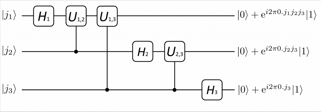
Figure 1: Three-qubit quantum Fourier transform circuit
In order to analyze this quantum circuit, the operators in Eq. (\eqref{315}) are next applied to the state $|j_{1}j_{2}j_{3}\rangle$ in a temporal order, first looking at the first qubit
\begin{equation}
H_{1}|j_{1}j_{2}j_{3}\rangle=\left(|0\rangle+e^{i 2\pi 0.j_{1}}|1\rangle\right)|j_{2}j_{3}\rangle\label{316}
\end{equation}
where the binary number $0.j_{1}$ represents the decimal $j_{1}/2$. When $j_{1}=0$, $e^{i 2\pi 0.j_{1}}=1$. When $j_{1}=1$, $e^{i 2\pi 0.j_{1}}=-1$. Specifically equation (\eqref{316}) can be expanded and written as:
\begin{equation}
\begin{aligned}
&U_{Q F T}|0\rangle=\frac{1}{\sqrt{2}}(|0\rangle+|1\rangle) \\
&U_{Q F T}|1\rangle=\frac{1}{\sqrt{2}}(|0\rangle-|1\rangle)
\end{aligned}
\end{equation}
One can see that this is the Hadamard transform, which is also the simplest Fourier transform. This is followed by the $\mathrm{C}(U_{1,2})$ operation, which does nothing when $j_{2}=0$, and then rotates the phase $\theta_{1,2}=2 \pi j_{2}/2^{2-1+1}=2 \pi0.0j_{2}$ to the first qubit $|1\rangle$ when $j_{2}=1$. This is followed by the $\mathrm{C}(U_{1,3})$ operation, which does nothing when $j_{3}=0$, and rotates the phase $\theta_{1,3}=2 \pi j_{3}/2^{3-1+1}=2 \pi0.00j_{3}$ for the first qubit $|1\rangle$ when $j_{3}=1$. The output state of the first qubit after this operation is:
\begin{equation}
\frac{1}{2^{1/2}}\left(|0\rangle+e^{i 2 \pi0.j_{1}j_{2}j_{3}}|1\rangle\right)
\end{equation}
The action of the quantum circuit on the second qubit is discussed below. $H_2$ acts after the second qubit
\begin{equation}
\frac{1}{2^{1/2}}\left(|0\rangle+e^{i 2\pi 0.j_{2}}|1\rangle\right)
\end{equation}
Immediately following the action $\mathrm{C}(U_{2,3})$ operation, when $j_{3}=0$ no operation is done, and when $j_{3}=1$ the phase is rotated $\theta_{2,3}=2 \pi j_{2}/2^{3-2+1}=2 \pi0.0j_{3}$ for the second qubit $|1\rangle$. At this point the quantum state evolves as:
\begin{equation}
\frac{1}{2^{1/2}}\left(|0\rangle+e^{i 2\pi 0.j_{2}j_{3}}|1\rangle\right)
\end{equation}
Finally, $H_3$ acting on the third qubit results in
\begin{equation}
\frac{1}{2^{1/2}}\left(|0\rangle+e^{i 2\pi 0.j_{3}}|1\rangle\right)
\end{equation}
Thus the quantum circuit prepared quantum states are
\begin{equation}
\frac{1}{2^{3/2}}\left[\left(|0\rangle+e^{i 2 \pi0.j_{1}j_{2}j_{3}}|1\rangle\right)\left(|0\rangle+e^{i 2\pi 0.j_{2}j_{3}}|1\rangle\right) \left(|0\rangle+e^{i 2\pi 0.j_{3}}|1\rangle\right)\right]
\end{equation}
Comparison with Eq.\eqref{311} reveals that this is exactly the Fourier transform of three qubits. This result can be generalized to the circuit of $n$ qubits. It will be shown below that the realizes the Fourier transform of Eq.\eqref{311} for $n$ qubits.
3.3. $n$-qubit quantum Fourier transform
The input state is $|j\rangle=|j_{1}j_{2},,,j_{n}\rangle$. The $H_1$ action on the state $|j\rangle$ results in:
\begin{equation}
\frac{1}{2^{1/2}}\left(|0\rangle+e^{i 2\pi 0.j_{1}}|1\rangle\right)|j_{2}j_{3}…j_{n}\rangle
\end{equation}
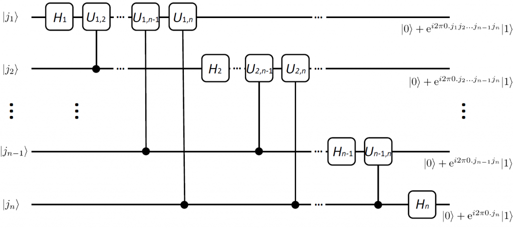
Figure 2: Circuit of n-qubit Quantum Fourier transform algorithm
Immediately after that act the $\mathrm{C}(U_{1,2})$ operation, doing nothing when $j_{2}=0$, and rotating the phase $\theta_{1,2}=2 \pi j_{2}/2^{2-1+1}=2 \pi0.0j_{2}$ to the first qubit $|1\rangle$ when $j_{2}=1$. This is followed by the $\mathrm{C}(U_{1,3})$ operation, which does nothing when $j_{3}=0$, and rotates the phase $\theta_{1,3}=2 \pi j_{3}/2^{3-1+1}=2 \pi0.00j_{3}$ for the first qubit $|1\rangle$ when $j_{3}=1$. . Then $\mathrm{C}(U_{1,3}), \mathrm{C}(U_{1,4}),\cdots$ are applied until $\mathrm{C}(U_{1,n})$. The output state of the first qubit after this operation is:
\begin{equation}
\frac{1}{2^{1/2}}\left(|0\rangle+e^{i 2 \pi0.j_{1}j_{2}\cdots j_{n}}|1\rangle\right)|j_{2}j_{3}…j_{n}\rangle
\end{equation}
Afterwards the operations $H_{2}, \mathrm{C}(U_{2,3}), \mathrm{C}(U_{2,4}), \cdots, \mathrm{C}(U_{2,n})$ are performed on the second qubit to get
\begin{equation}
\frac{1}{2}\left(|0\rangle+e^{i 2 \pi0.j_{2}j_{3}\cdots j_{n}}|1\rangle\right)\left(|0\rangle+e^{i 2 \pi0.j_{1}j_{2}\cdots j_{n}}|1\rangle\right)|j_{3}j_{4}…j_{n}\rangle
\end{equation}
Follow the quantum circuit for each qubit in turn until the $n$-th qubit. The final result is obtained as
\begin{equation}
\frac{1}{2^{n / 2}}\left(|0\rangle+e^{2 \pi i 0 . j_{n}}|1\rangle\right)\left(|0\rangle+e^{2 \pi i 0 . j_{n-1} j_{n}}|1\rangle\right) \cdots\left(|0\rangle+e^{2 \pi i 0 . j_{1} j_{2} \cdots j_{n}}|1\rangle\right)
\end{equation}
This is exactly the result of Eq.\eqref{311}. Thus it is proved that the Figure 2 is the circuit of the $n$-qubit quantum Fourier transform.
Analyzing this algorithm shows that for an $n$-qubit circuit the logic gates applied sequentially are
\begin{equation}
H_{n} \mathrm{C}(U_{n-1,n})H_{n-1} \mathrm{C}(U_{n-2,n-1})\cdots H_{2} \mathrm{C}(U_{1,n}) \mathrm{C}(U_{1,n-1})\cdots \mathrm{C}(U_{1,2})H_{1}
\end{equation}
A total of $n$ $H$ gate operations and $\frac{n(n-1)}{2}$ two-qubit gate operations were applied. A total of $\frac{n(n+2)}{2}$ operations are performed, and it can be seen that the total number of operations required is a quadratic function of the number of input qubits. Thus the complexity of the quantum Fourier transform is $\Theta\left(n^2\right)$, while the best classical Fourier transform algorithm has a complexity of $\Theta\left(n2^n\right)$.