1. Loading classical data: quantum state preparation
To process classical data with quantum algorithm, the first step is to encode the classical information to the wavefunction of a quantum system. The most widely used encoding method is called amplitude encoding. It is equivalent to the task of \textbf{quantum state preparation} (QSP). Suppose we are given a normalized vector $\alpha=[\alpha_0,\cdots,\alpha_{N-1}]$. Without loss of generality, we assume that $N=2^n$ with $n$ an integer. The task is to generate a quantum state
\begin{align}\label{bl_eq:targ}
|\psi_{\text{target}}\rangle=\sum_{k=0}^{2^n-1}\alpha_k|k\rangle.
\end{align}
Here, $|k\rangle$ denotes an $n$-qubit bitstring. For example, If $n=3$, $j=2$, we have $|k\rangle=|010\rangle$. Without loss of generality, we assume that the initial quantum state is at a trivial, non-entangled state $|0\cdots0\rangle$.
1.1. Long-Sun-Grover-Rudolph algorithm Naively, constructing an arbitrary $n$-qubit unitary requires $O(4^n)$ elementary quantum gates. But it turns out that the complexity of QSP is much smaller. The first nontrivial algorithm for QSP is proposed by Long and Sun at 2001~[1], and proposed independently by Grover and Rudolph at 2002~[1]. The algorithm works as follows.
For simplicity, we assume that all amplitudes to be real, i.e. $\alpha_k\in \mathbb{R}$, while the generalization to complex value cases is straightforward. The LSGR algorithm works in a divide-and-conquer way. We define $\alpha_{n,k}\equiv\alpha_k$, and iteratively, $\alpha_{j,k}\equiv\sqrt{\alpha_{j-1,2k}^2+\alpha_{j-1,2k+1}^2}$ for $1\leq j\leq n$. Let ${\alpha_j}=[\alpha_{j,0},\cdots,\alpha_{j,2^{j}}]$. We define a single-qubit rotation
\begin{align}
R(\theta)=\begin{pmatrix}\cos\theta&-\sin\theta\\\sin\theta&\cos\theta
\end{pmatrix}.
\end{align}
It can be verified that $R(\theta)|0\rangle=\cos\theta|0\rangle+\sin\theta|1\rangle$. So if we define $\theta_{1,0}=\arccos\alpha_{1,0}$, and implement $R(\theta_{1,0})$ at initial state $|0\rangle$, we obtain
\begin{align}
R(\theta_{1,0})|0\rangle=\alpha_{1,0}|0\rangle+\alpha_{1,1}|1\rangle.
\end{align}
Similarly, for $j>1$, we define $\theta_{j,k}=\arccos\frac{\alpha_{j,2k}}{\alpha_{j-1,k}}$ for $0\leq k\leq 2^{j-1}$, and ${\theta}_j=[\theta_{j,0},\cdots,\theta_{j,2^{j-1}}]$. We introduce a multi-qubit controlled rotation
\begin{align}
CR({\theta_j})\sum_{k=0}^{2^{j-1}}|k\rangle\langle k|\otimes R(\theta_{j,k}).
\end{align}
At the $j$th step, suppose we have obtained a $j$-qubit quantum state $\sum_{k=0}^{2^j-1}\alpha_{j,k}|k\rangle$, we introduce a extra qubit, and implement the uniformly controlled rotation $CR({\alpha_j})$, and obtain
\begin{align}
CR({\theta_j})\sum_{k=0}^{2^j-1}\alpha_{j,k}|k\rangle|0\rangle&=\sum_{k=0}^{2^j-1}\alpha_{j,k}|k\rangle(\cos\theta_{j,k}|0\rangle+\sin\theta_{j,k}|1\rangle)\\
&=\sum_{k=0}^{2^{j+1}-1}\alpha_{j,k}|k\rangle
\end{align}
After the $n$th step, we obtain the quantum state $\sum_{k=0}^{2^n-1}\alpha_{n,k}|k\rangle=\sum_{k=0}^{2^n-1}\alpha_{k}|k\rangle$. An example for $2$-qubit state preparation is illustrated in Fig 1
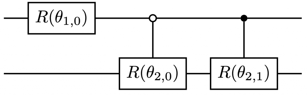
Fig 1: Sketch 2-qubit state preparation protocol
At the $j$th step, each many-qubit controlled rotation requires $O(j)$ elementary quantum gates. One can decompose $CR({\theta_j})$ into $2^j$ many-qubit controlled gates. Therefore, the $j$th step accounts for totally $O(j2^j)$ gate complexity, and the total gate complexity of QSP is $\sum_{j=1}^n=O(j2^j)=O(n2^n)$. It is worthy to note that there are nontrivial way of implementing $CR({\theta_j})$ with gate complexity $O(2^j)$. Readers are refereed to~[1] for more details.
1.2. Plesch-Brukner algorithm~[1]
We assume that the number of qubits $n$ is an even. To begin with, we can divide all qubits into two parts (denoted as $A$ and $B$), each with $n$ qubits. We can always rewrite $|\psi_{\text{targ}}\rangle$ in the Schmidt decomposition form,
\begin{align}\label{bl_eq:pb1}
|\psi_{\text{targ}}\rangle=\sum_{k=0}^{2^{n/2}-1}\alpha_k|\psi_A\rangle_k|\psi_B\rangle_k
\end{align}
for some $n/2$-qubit orthonormal basis $\{|\psi_A\rangle_k\}$ and $\{|\psi_B\rangle_k\}$. With initial state $|0\rangle^{n}$, we first perform the transformation
\begin{align}\label{bl_eq:pb2}
|0^n\rangle\rightarrow\sum_{k=0}^{2^{n/2}-1}\alpha_k|k_A\rangle|0^{n/2}_B\rangle.
\end{align}
In the second step, we perform CNOT gate with qubits at part $A$ (B) as control (target) qubits,
\begin{align}\label{bl_eq:pb3}
\sum_{k=0}^{2^{n/2}-1}\alpha_k|k_A\rangle|0^{n/2}_B\rangle\longrightarrow\sum_{k=0}^{2^{n/2}-1}\alpha_k|k_A\rangle|k_B\rangle.
\end{align}
In the third step, we apply two unitaries $U_A=\sum_{k}|\psi_A\rangle_k\langle k_A|$ and $U_B=\sum_{k}|\psi_B\rangle_k\langle k_B|$, achieving the final target state
\begin{align}\label{bl_eq:pb4}
\sum_{k=0}^{2^{n/2}-1}\alpha_k|k_A\rangle|k_B\rangle\xrightarrow[]{U_A\otimes U_B} \sum_{k=0}^{2^{n/2}-1}\alpha_k|\psi_A\rangle_k|\psi_B\rangle_k=|\psi_{\text{targ}}\rangle.
\end{align}
The QSP problem for $n$ qubit state is then decomposed into to the QSP for two $(n/2)$ qubit state and a unitary synthesis problem of $n/2$-qubit system. Such decomposition process can be constructed recursively. The dominant contribution of gate complexity is from the unitary synthesis step (Eq.~\eqref{bl_eq:pb4}). The $n/2$-qubit unitary synthesis requires totally $O(4^{n/2})=O(2^n)$ single- and two-qubit gates. Therefore, the complexity of the Plesch-Brukner algorithm is also $O(2^n)$.
2. Quantum random access memory
In analogy to the classical random access memory, quantum random access memory aims at performing the following transformation~[1]
\begin{align}\label{bl_eq:qram}
U_{\text{QRAM}}|j\rangle_{\text{L}}|0\rangle_{\text{W}}=|j\rangle_{\text{L}}|D_j\rangle_{\text{W}},
\end{align}
for some $D_j\in\{0,1\}$. Here, L represents an $n$-qubit label register, and D represents the word register, typically with one classical bit. In general, performing the transformation Eq.~\eqref{bl_eq:qram} requires $O(2^n)$ elementary quantum gate. This means that a naive construction Eq.~\eqref{bl_eq:qram} requires exponential runtime. However, we may introduce ancillary qubits to trade space for runtime. It turns out that with $O(2^n)$ ancillary qubits, we can realize Eq.~\eqref{bl_eq:qram} with $O(n)$ runtime.
2.1. Bucket-Brigade QRAM There are many ways of implementing QRAMs. One of the simplest implementation is the Bucket-Brigade QRAM (BBQRAM), which requires only geometrically local quantum gates, and does not require multi-qubit controlled rotations. In below, we introduce one of the circuit implementation of it based on qubit.
The element of the BBQRAM is the router containing four qubits. Its incident qubit (inc), routing qubit (rou), left output qubit (left) and right output qubit (right). the router operation performs the following transformation.
\begin{align}\label{eq:routing}
\text{ROUTE}|\psi\rangle_{\text{inc}}|0\rangle_{\text{rou}}|0\rangle_{\text{right}}|0\rangle_{\text{left}}=|0\rangle_{\text{inc}}|0\rangle_{\text{rou}}|\psi\rangle_{\text{right}}|0\rangle_{\text{left}}\\
\text{ROUTE}|\psi\rangle_{\text{inc}}|1\rangle_{\text{rou}}|0\rangle_{\text{right}}|0\rangle_{\text{left}}=|0\rangle_{\text{inc}}|0\rangle_{\text{rou}}|0\rangle_{\text{right}}|\psi\rangle_{\text{left}}
\end{align}
In other words, the state of incident qubit is transferred to the left (right) qubit, if the routing qubit is at state $|0\rangle$ ($|1\rangle$).
The layout of BBQRAM is shown in Fig 2. The layout contains ($2d-1$) routers arranged as an $n$-layer binary tree. Each left (right) output qubit serves as the incident qubit of its left (right) child. Each left and right output qubit of the node at the leaf layer connects to a memory cell. The $j$th memory cell contains one classical bit initialized as $|D_j\rangle$.
We begin by applying a Hadamard gate at data qubit, so the state becomes $|j\rangle_\text{L}|+\rangle_\text{W}$. The BBQRAM then contains three stages.
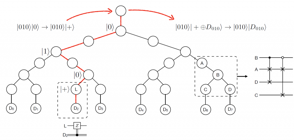
Fig 2: Sketch of BBQRAM
Route-in stage. The state of index register and data register qubits are sent into the binary tree sequentially. ROUTE defined by Eq.~\eqref{eq:routing} transfers the state of the incident qubit of a node to the incident qubit of its left (right) child, conditioned on the routing qubit is at state $|0\rangle$ ($|1\rangle$). With a swap gate, the state of the $l$th index qubit is finally transferred to one of the routing qubits at the $l$th layer. The states of the word qubit ($|+\rangle$) is send into the $j$th leaf node, while all other leaf nodes remains at state $|0\rangle$. This stage requires $O(n)$ layer of single- and two-qubit gates.
Query stage. In the query stage, we apply totally $2^n$ controlled phase gates in parallel, each with the $j$ data bit as controlled bit, and the $j$th leaf qubit as target qubit. This gives the transformations $|+\rangle|D_j\rangle\rightarrow|+\oplus D_j\rangle|D_j\rangle$ and $|0\rangle|D_{j’\neq j}\rangle\rightarrow|0\rangle|D_{j’\neq j}\rangle$. Here, we have defined $|+\oplus\; 0\rangle=|+\rangle$ and $|+\oplus\; 1\rangle=|-\rangle$.
Route-out stage. In the route-out stage, we perform the inverse of the route-in stage. The binary tree will then be uncomputed, all qubits of which will return to the initial state $|0\rangle$. Meanwhile the label and data qubit becomes $|j\rangle_{\text{L}}|+\oplus\; D_j\rangle_\text{W}$. We apply Hadamard gate at the data qubit, the state then becomes $|j\rangle_\text{L}|D_j\rangle_\text{W}$ as expected.
An example is given in Fig 2, where the index register is initially as $|010\rangle$.
2.2. Generalized QRAM
QRAM defined in Eq.~\eqref{bl_eq:qram} can load data to a classical system with high speed. However, it does not work for general data when $|D_j\rangle$ is a superposition of $|0\rangle$ and $|1\rangle$. So its applications are restricted. We may generalize the definition of QRAM to continuous, high-dimensional data
\begin{align}\label{bl_eq:gqram}
U_{\text{QRAM}}|j\rangle_\text{L}|0\rangle_\text{W}=|j\rangle_\text{L}|\psi_j\rangle_\text{W}
\end{align}
where $|\psi_j\rangle\in\mathbb{C}^{2^m\times 2^m}$ is an $m$ qubit normalized quantum state. In this case, if we still use the process introduced in previous section, the binary tree will not be fully uncomputed. This is because at the query stage, there is no way to prepare the $j$th leaf node a an appropriate state, while keeping all other leaf node unchanged (note that the value of $j$ is unknown).
This problem can be solved by introducing an extra pointer qubit. We provide a detailed implementation at Appendix.
3. Block encoding In quantum computing, the transformation given by the quantum circuits are unitaries. Therefore, one can not perform general linear transformation on a given input data (quantum state). However, we can embed a general matrix, after rescaling, to a unitary in a higher dimension. In this way, one may perform a general transformation effectively. This technique, called block-encoding, has broad applications in Hamiltonian simulation, linear algebra tasks etc.
We say that $O_A$ is the block encoding of $A$ if
\begin{align}
(\langle\tilde\psi|\otimes I)O_A(|\psi\rangle\otimes I)=A
\end{align}
for some easily prepared quantum states $|\psi\rangle$ and $|\tilde\psi\rangle$. As a simplest case, we may choose the computational basis, and set $|\psi\rangle=|\tilde\psi\rangle=|0^a\rangle$. In this case, the matrix form of $O_A$ is as follows
\begin{align}
O_A=\begin{pmatrix}A&\cdot\\\cdot&\cdot
\end{pmatrix}.
\end{align}
The non-unitary matrix $A$ is encoded at the upper left block of a larger unitary matrix $O_A$, and this is the origin of the name “block-encoding”.
To ensure that $O_A$ is a unitary, it is required that the $L_2$ norm of matrix $A$ is bounded by $1$, i.e. $\|A\|_2\leq1$. If this is not the case, we can rescale the matrix $A$ and perform the block encoding of $A/\alpha$ for some $\alpha\geq\|A\|_2$.
4. General matrix
We introduce two $n$-qubit registers, denoted as $A$ and $B$. We then suppose that we have two unitaries $U_R$ and $U_L$ satisfying the following
\begin{align}
U_R|0^n\rangle_A|j\rangle_B&=|\psi_j\rangle_A|j\rangle_B\\
U_L|0^n\rangle_A|k\rangle_B&=|k\rangle_A|\psi_k\rangle_B,
\end{align}
where
\begin{align}
|\psi_j\rangle=\sum_{k=0}^{N-1}\frac{A_{j,k}}{\|A_{j,\cdot}\|},\quad
|\phi_k\rangle=\sum_{j=0}^{N-1}\frac{\|A_{j,\cdot}\|}{\|A\|_F}.
\end{align}
Here, $A_{j,\cdot}\equiv[A_{j,0},A_{j,1},\cdots,A_{j,N-1}]$ is the $j$th row of matrix $A$, $\|\cdot\|$ is the Euclidean norm of vectors, and $\|\cdot\|_F$ is the Frobenius norm of matrix. Note that $|\phi_k\rangle$ is independent of $k$, so it is equivalent to a QSP unitary, up to a swap between registers $A$ and $B$. Besides, $U_R$ is a generalized QRAM as defined in Eq.~\eqref{bl_eq:gqram}. Let $U_A=U_R^{+} U_L$, it can be verified that
\begin{align}
\langle 0^n|_A\langle j|_BU_A|0^n\rangle_A|k\rangle_B=\frac{A_{j,k}}{\|A\|_F},
\end{align}
and equivalently,
\begin{align}
\langle 0^n|_AU_A|0^n\rangle_A=\frac{A}{\|A\|_F},
\end{align}
Therefore, $U_A$ is a block encoding of $\frac{A}{\|A\|_F}$.
5. Linear combination of untiaries
Linear combination of untiaries (LCU) is a simple way to perform block encoding. We assume that matrix A has been decomposed as
\begin{align}
A=\sum_{j=1}^J\alpha_jV(j),
\end{align}
for some efficiently implementable unitaries $V(j)$ and positive value $\alpha_j>0$. Let $\alpha=\sum_{j=1}^J\alpha_j$, we define $G$ as a quantum state preparation unitary such that
\begin{align}
G|0^a\rangle=\sum_{j=1}^J\sqrt{\frac{\alpha_j}{\alpha}}|j\rangle.
\end{align}
Then we introduce the select oracle
\begin{align}
\text{Select}(V)=\sum_{j=1}^J|j\rangle\langle j|\otimes V(j).
\end{align}
We consider an $n+\lceil\log_2J\rceil$ qubit system, and define
\begin{align}
O_{\tilde A}=G^{+}\text{Select}(V)G.
\end{align}
It can be verified that
\begin{align}
\langle0^{\lceil\log_2J\rceil}| G^{+}\text{Select}(V)G|0^{\lceil\log_2J\rceil}\rangle=A/\alpha.
\end{align}
Therefore, $G^{+}\text{Select}(V)G$ is a block-encoding of $A/\alpha$.
$G$ and $G^{+}$ can be implemented with $O(J)$ single- and two-qubit gates, Select(V) can be implemented with $O(J)$ queries to $V_j$ and $O(J)$ extra single- and two-qubit gates. Therefore, when $J=O(\text{Poly}(n))$, the block encoding $O_{\tilde A}$ can be constructed with polynomial-size quantum circuit.
6. History and further Reading Quantum state preparation. After Ref~[1], the gate complexity of state preparation is then improved to $O(2^n)$ by [1] and various other proposals~[1]. The fundamental lower bound $\Theta(2^n/n)$ was achieved by~[1]. By introducing ancillary qubits, the state preparation circuit depth can be reduced significantly. There are several works achieving $O(n)$ circuit depth using $O(2^n)$ or $\tilde O(2^n)$ ancillary qubits. Ref.~[1] use a QRAM-like binary tree architecture with sparse connectivity, while other works assumes all-to-all connectivity. Ref.~[1] allows space-time trade-off with arbitrary number of ancillary qubits. The state preparation complexity can also be reduced when the target state has certain structures. For example, for sparse quantum state with $d$ nonzero entries, the circuit depth can be reduced to $O(nd)$ with $O(1)$ ancillary qubits~[1] or $O(\log(nd))$ with $O(nd)$ ancillary qubits~[1].
Quantum Random Access memory. QRAM is first proposed in Ref.~[1]. The generalization to nonbinary data is first proposed in~[1], which maintains the original sparse connectivity of QRAM architecture. Ref.~[1] first show how Eq.~\eqref{bl_eq:gqram} can be constructed for general $|\psi_j\rangle$, although their method requires all-to-all connectivity. There proposal also allows space-time trade-off with arbitrary ancillary qubits. Readers may be referred to~[1] for a comprehensive review of QRAM.
Block encoding. The idea of block-encoding is first proposed in Ref.~[1], with the name the standard-form encoding. Ref.~[1] introduces the applications in Hamiltonian simulation, with optimal query complexity. “Block-encoding” is named after~[1], which introduce other applications, such as singular value estimation, and solving linear system. There are some other methods for Block-encoding construction~[1], such as based on sparse-access input model, and Purified Density Matrix. These methods are based on some special quantum oracles.